Bayesian Estimation in Action
Hello All, In this post I will demonstrate a practical use case of applying Bayesian Estimation in a typical business scenario. Quite often businesses are required to take decisions based on some analysis of observed data. We will see how Bayesian Estimation becomes a very important tool to help us quantify the uncertainty in the data and help us take more informed decisions.
Problem Definition
Let’s consider a situation where one needs to decide whether to broad-base a certain Ad or an emailer to the target segment. We will also consider that by showing the Ad/emailer to a test sample of 100 customers resulted in a total conversion of 8 customers.
Now the team is faced with the following questions.
1. What would be the expected conversion if the ad/emailer is shown to the entire segment?
2. Suppose, there is a proven channel which guarantees a conversion rate of 3%. What is the probability that the conversion rate of this new ad/emailer is greater than 3%?
3. What will be the total number of conversions if the ad/emailer is shown to 200K consumers?
From the back of the envelope calculation, we can say that the expected conversion rate is 8% (8/100). But what is the certainity of this estimate? This is where Bayesian Estimation helps us to identify the conversion estimate and quantify the uncertainty in the estimate. We can use various computation methods for Bayesian Estimation. In this post I will show two different methods. Approxmiate Bayesian Computation (ABC) and MCMC. For the latter method I will use the Stan (more later).
So let’s get started with the first problem.
Bayesian Estimation using ABC
1. What would be the expected conversion if the ad/emailer is shown to the entire population?
To solve this question, we need to develop a model based on the observed data. The Bayesian modeling consists of 3 components:
i. Data
ii. A generative model
iii. Prior belief of the parameters
Typically, we start by defining the parameters and building the generative model. A generative model is defined as a probability model which can stochastically generate data using a set of parameters. The observed data is an instance of the generative model.
Let’s say there is an underlying success rate parameter θ which is an unknown and defined as the probability of conversion. Each customer decides to conver or not convert at this rate. We are trying to ultimately find out the distribution of this success rate parameter. To begin with, we assume that θ is uniformly distributed as we do not know any prior information of θ. Often times this is called uninformative prior as a uniform distibution gives equal credibility to all values between 0 and 1.
We randomly sample a value of θ from the uniform distribution and use this value as input to the generative model. The generative model outputs the total conversion (number of successes) given the success rate parameter and number of trials (100 in this case). The generative model can be a binomial distribution for example. We repeat this experience say 100000 times.
Below is the code for this simulation.
# Number of experiments
ndraws <- 100000

# Pick the success rate from Uniform distribtuion
prior_rate <- runif(ndraws, 0, 1)

#Define the generative model
genmodel <- function(rate) {
        rbinom(n = 1, size = 100, prob = rate)
}

# Pass the success rate to generative model
conversions <- sapply(prior_rate, function(x) genmodel(x))
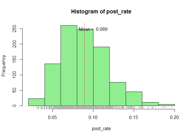
Now comes the interesting part, out of the 100000 experiements we will filter out those experiments which resulted in our actual data i.e. 8 conversions out of 100 customers. The distribution of the sucess rates which resulted in the actual data is defined as the posterior distribution and is the output of the Bayesian Estimation.
# Filter rates which resulted in the actual data i.e. 8 conversions out of 100 customers
post_rate <- prior_rate[conversions == 8]

# Distribution of the resulting success rates
hist(post_rate, col = "lightgreen")
abline(v = mean(post_rate), lty = 2, col = "red")
rug(post_rate, col = "gray70")
text(x = 0.1, y = 250, paste("Mean = ", round(mean(post_rate), 3)))

Once we have the posterior distribution of the success rate we can derive lot of value from it. Like the mean and 95% (Credible Interval) of the success rate and also answer our questions.
The expected value of the coversion is the mean of the posterior distribution.
mean(post_rate)

## [1] 0.08918136
The expected conversion rate is 8.92% which is slightly different from our back of the envelope estimate.
Below is the 95% CI
quantile(post_rate, c(0.025, 0.975))

##       2.5%      97.5%
## 0.04064573 0.15577722
In other words we can be 95% confident that the conversion rate lies between 4.1% and 15.6%.
Note that we considered an uniform distribution for the prior as we had no clue about its previous distribution. The prior can have any distribution based on the previous knowledge about the parameters.
2. Suppose, there is a proven channel which guarantees a conversion rate of 3%. What is the probability that the conversion rate of this new ad/emailer is greater than 3%?
This can be easily obtained from the probability distribution.
sum(post_rate > 0.03)/length(post_rate)

## [1] 0.998995
We can be 99.9% confident that the Ad/emailer will have a total conversion greater than 3%.
3. What will be the total number of conversions if the ad/emailer is shown to 200K consumers?
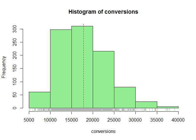
Again, this is can be done easily as we now have the distribution of the conversion rate. We simulate the data using the binomial function.
conversions <- rbinom(n = length(post_rate), size = 200000, prob = post_rate)
hist(conversions, col = "lightgreen")
abline(v = mean(conversions), lty = 2, col = "red")
rug(conversions, col = "gray70")

quantile(conversions, c(0.025, 0.975))

##    2.5%   97.5%
##  8185.3 31267.5
With 95% we can say that that total conversions lies between 8186 to 3.126710^{4} customers.
I hope by now you can appreciate how simple Bayesian Estimation can serve business insights. The approach of simulation we followed above is called Approximate Bayesian Estimation. This method is very intuitive and easy to simulate. But this approach falls flat when the model complexity increases as it requires huge computational resources. Therefore the need to move towards effective methods like MCMC which adapt certain computational shortcuts while doing simulations.
Bayesian Estimation Using Stan
We will replicate the above experiment using the rstan package in R.
Stan is a domain specific probabilistic programming language to be used
in tandem with other languages like R. Stan allows us to draw samples
from the parameter space once we specify the details like data,
generative model and priors.
In R, we prepare a string with Stan syntax. Inside the string, we
declare the data, parameters and define the model. Our data is a
binomial experiment with n trials and s successes. We have only one
parameter (the underlying success rate). Inside the model block we
define random draws from a uniform distribution for the success rate and
this rate is used to perform a binomial trial to generate the data.
library(rstan)

# The Stan model as a string.
model_string <- "
# Here we define the data we are going to pass into the model
data {
  int n; # Number of trials
  int s;  # Number of successes
}

# Here we define what 'unknowns' aka parameters we have.
parameters {
  real<lower=0, upper=1> rate;
}

# The generative model
model {
  rate ~ uniform(0, 1);
  s ~ binomial(n, rate);
}
"
After defining the model string, we define the observed data and start the simulation process.
The object stan_samples consists of samples from posterior
distribution of the parameter space. In this case it consists of
multiple values of θ which resulted in the observed data.
Lets take a look at the stan-samples object.
stan_samples

## Inference for Stan model: d7fc75d5f2b6fc44fca1059e978887ae.
## 4 chains, each with iter=2000; warmup=1000; thin=1;
## post-warmup draws per chain=1000, total post-warmup draws=4000.
##
##        mean se_mean   sd   2.5%    25%    50%    75%  97.5% n_eff Rhat
## rate   0.09    0.00 0.03   0.04   0.07   0.09   0.11   0.15  1979    1
## lp__ -30.93    0.01 0.68 -32.81 -31.13 -30.66 -30.49 -30.44  2248    1
##
## Samples were drawn using NUTS(diag_e) at Tue May 16 17:46:27 2017.
## For each parameter, n_eff is a crude measure of effective sample size,
## and Rhat is the potential scale reduction factor on split chains (at
## convergence, Rhat=1).
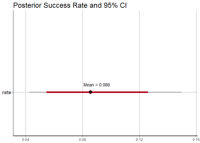
We can observe that the mean or estimated success rate is 8.8% which is very similar to what we obtained using the ABC method. Also, a total of 4 MCMC chains have been constructed to arrive at this value.
The 95% Credible Interval is 4% to 15% which again matches with our earlier simulation.
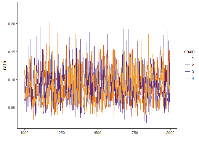
The below traceplot function plots the movement of the success rate
parameter during the MCMC process. This plot can be used as one of many
sanity checks to validate if the simulation was stable and did not get
stuck.
traceplot(stan_samples)

Below we can see the success rate represented by a dot and the 95% CI around it.
plot(stan_samples) +
        annotate("text", x= 0.09, y = 1.1, label = paste("Mean =", round(mean(as.data.frame(stan_samples)$rate),3))) +
        labs(title = "Posterior Success Rate and 95% CI")

Conclusion
In this post we have see how Bayesian Estimation can be applied to real world problems for decision making. Bayesian Estimation is a very effective tool to quantitatively describe uncertainity in the data. But we have not even scratched the surface of what can possibly be done using Bayesian Estimation. In the following posts I will show how we can use Bayesian methods for A/B testing, build more complex models and use predict outcomes.